2017-03-07: The spatial variability of the surface mass loss of the Greenland ice sheet affects the entire ocean !
Summary
Mass loss from the Greenland ice sheet – surface and basal melting of snow & ice, and iceberg discharge, consequence of the positive Earth’s energy imbalance and its associated increase in surface temperature – is an important contributor to the current sea level rise, i.e. around 18% of the global mean sea level rise during the last two decades, and is expected to accelerate during the twenty-first century (Church et al., 2013). The mass loss at the surface – approximated by the difference between snowfall and snow melting, called surface mass balance (SMB) – is expected to dominate the entire mass loss of the Greenland ice sheet at the end of this century (Goelzer et al., 2013). The mass redistribution (transferred from Greenland ice sheet into ocean) associated with Greenland SMB generates changes in sea level through the influence on the Earth’s gravitational field, the Earth rotation axis and the crust deformation. The 5th Intergovernmental Panel of Climate Change (IPCC) report projected sea level rise at global and regional scale associated with Greenland SMB over the 21st century. However, the last IPCC report did not take into account the regional variability in Greenland surface mass balance.
In a recent study, researchers from the Laboratoire d’Etudes en Géophysique et Océanographie Spatiale (LEGOS) and the Université of Liège , which are members of the international team of the International Space Science Institute (ISSI) on “Contemporary global and regional sea level rise” (http://www.issibern.ch/teams/climatemodels/), studied the regional sea level changes in response to the surface mass loss of the Greenland ice sheet. They showed that the Greenland SMB changes show a large regional variability due to different climatic conditions, snow & ice properties, and surface elevation & geometry over the Greenland basins (Figure 1 & 2). They found that the southern part of Greenland is more sensitive to climate warming, and thus that its surface mass balance will decrease sooner in the twenty-first century that the northern part (Figure 1 & 2). This regional variability in Greenland surface mass balance results in spatial variability of sea level changes over the entire ocean, and has to be taken into account in sea level projections, especially along the United State East coast and the northern coast of Europe (Figure 3 & 4) where the effect is the most important.
Method
The regional sea level changes associated with Greenland SMB changes are obtained using the sea level equation that describes sea level changes induced by melting of ice sheets (Farrell and Clark, 1976). In order to derive several estimates of Greenland surface mass balance – and also to study its effect on regional sea level – for each 6 major drainage basins (Figure 1) during the twenty and twenty-first centuries, this study used a downscaling technique calibrated against the Modèle Atmosphérique Régional (MAR) and forced by 32 climate models (from the Coupled Model Intercomparison Project phase 5 – CMIP5) over the 1900-2100 time period. For the twentieth century, historical climate simulations are used, and for the twenty-first century scenario RCP8.5 simulations are used. Comparison for the end of the twentieth century with MAR forced by ERA-40 and ERA-Interim climate reanalysis – considered as reference – shows a good agreement at decadal and multidecadal time scales. Over the twentieth and twenty-first centuries, the ensemble of Greenland surface mass balance estimates shows a significant decrease in all basins as the climate warms – projected Greenland surface contribution to global mean sea level rise in 2081–2100 is around 20 centimeters.
Remarks
Due to the expensive computational time, it was not possible to perform 32 MAR simulations forced by the 32 climate models. Consequently, a downscaling calibration approach what developed using 4 reference MAR simulations that served to empirically calibrate snowfall and runoff of the climate models.
It’s also important to note that “the results are probably conservative because the effects of ice sheet dynamics, ice sheet topography changes, the routing of surface water, and freshwater inputs on the ocean circulation are not taken into account. To go a step further and take these effects into account, we would need to couple the MAR regional climate model with an ice sheet model and dynamics model as well as with an ocean model.”
Main references
-
Alexander, P., Tedesco, M., Schlegel, N.-J., Luthcke, S., Fettweis, X. and E. Larour, 2016: Greenland Ice Sheet seasonal and spatial mass variability from model simulations and GRACE (2003–2012). The Cryosphere, Volume 10, pp 1259–1277.
-
Church, J. and Coauthors, 2013: Sea Level Change. Climate Change 2013: The Physical Science Basis, Stocker, T. et al., Cambridge University Press, pp 1137-1216.
-
Farrell, W. and J. Clark, 1976: On postglacial sea level. Geophys. J. Int., Volume 46, pp 647–667.
-
Fettweis, X., 2007: Reconstruction of the 1979–2006 Greenland ice sheet surface mass balance using the regional climate model MAR. The Cryosphere, Volume 1, pp 21–40.
-
Fetweiss, X., Franco, B., Tedesco, M., van Angelen, J., Lenaerts, J., van den Broeke, M. and H. Gallée, 2013: Estimating the Greenland ice sheet surface mass balance contribution to future sea level rise using the regional atmospheric climate model MAR. The Cryosphere, Volume 7, pp 469–489.
-
Goelzer, H. and Coauthors, 2013: Sensitivity of Greenland ice sheet projections to model formulations. J. Glaciol., Volume 59, pp 733–749.
-
Lenaerts, J., van den Broeke, M., van Angelen, J., van Meijgaard, E. and S. Dery, 2012: Drifting snow climate of the Greenland ice sheet: A study with a regional climate model. The Cryosphere, Volume 6, pp 891–899.
-
Mitrovica, J., Tamisiea, M., Davis, J. and G. Milne, 2001: Recent mass balance of polar ice sheets inferred from patterns of global sea-level change. Nature, Volume 409, pp 1026–1029.
Figures
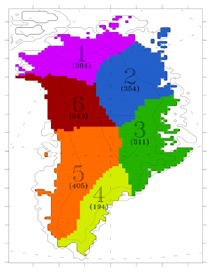 Figure 1. Map of the Greenland drainage basins.
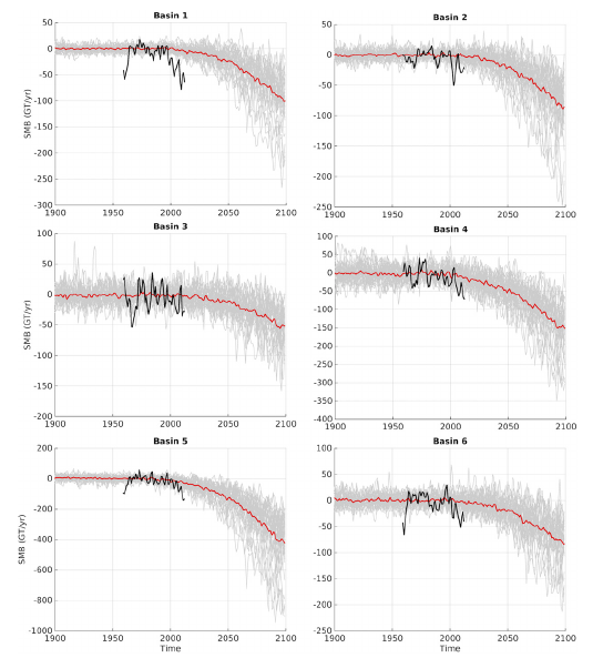
Figure 2. Annual surface mass balance anomalies (in Gt yr–1, scaling with the 1970-89 period) calculated with the regional atmospheric model MAR, forced by 32 climate models using the downscaling approach (individual model simulations are in gray and the ensemble mean is the red line) and forced by ERA-40 & ERA-Interim reanalysis (black curve) for basins 1, 2, 3, 4, 5, and 6.
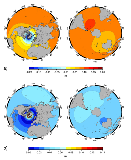
Figure 3. Ensemble mean (a) & standard deviation (b) of the regional relative sea level changes over 2080-2099 (with respect to 1900-1919) in response to Greenland SMB changes as estimated by the downscaling technique forced by global climate model outputs (see text). The regional sea level patterns of (a) & (b) include the effect of the regional variability in Greenland SMB changes.
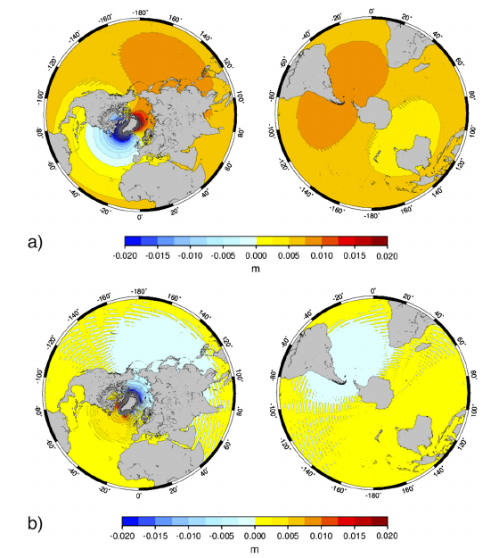 Figure 4. Ensemble mean (a) & standard deviation (b) of the regional relative sea level changes over 2080-2099 due to the regional variability in the Greenland SMB changes only.
Links
- >>> Outreach in pdf
- >>> Paper in pdf – Meyssignac, B., Fettweiss, X., Chevrier, R. and Spada, G. (2017). Regional Sea Level Changes for the Twentieth and the Twenty-First Centuries Induced by the Regional Variability in Greenland Ice Sheet Surface Mass Loss, Journal of Climate.
2016-05-03: Explanation of the thermal expansion differences across climate models !
Summary
More than 90% of the positive Earth’s energy imbalance – mainly anthropogenic as origin (Church et al. 2013) – is stored in the ocean as heat. Ocean warming results in thermal expansion and finally converts into sea level rise. During the last century, around half of the rate of sea level rise – globally averaged – was due to thermal expansion, called thermosteric sea level. For the coming century, Earth’s energy imbalance is expected to be constant or to increase, depending of human activity scenarios. Consequently, sea level rise is expected to be constant or to increase, and projection accuracy of sea level is dependent on the ability of climate models to predict ocean thermal expansion.
In a recent study, two researchers from the Laboratoire d’Etudes en Géophysique et Océanograohie Spatiales (LEGOS), which are members of the international team of the International Space Science Institute (ISSI) on “Contemporary global and regional sea level rise” ( http://www.issibern.ch/teams/climatemodels/ ), compare the thermal expansion obtained by climate models (from the Coupled Model Intercomparison Project phase 5), driven by atmospheric re-analyses, with observations over the period 1961 – 2005. The ensemble mean of sea level rise due to ocean warming from climate models is close to the observations – within observation uncertainty – in terms of absolute sea level rise as well as of rate of sea level rise (see Figure 1). However, the model ensemble exhibits a large spread. The authors then aim to explain this climate model spread over the twentieth and twenty-first centuries.
By deriving the Earth energy budget – under the condition of continuously increasing radiative forcing F – the authors show that the thermosteric part of sea level rise depends linearly on the time-integrated radiative forcing, which represents the total energy accumulated into the Earth system due to the current positive Earth’s energy imbalance. The linear relationship between thermosteric sea level rise and time-integrated F is confirmed by climate models under transient climate change like during the 20th century or the 21st century (under rcp4.5 and 8.5 scenarios). The constant of proportionality μ between time-integrated F and thermosteric sea level rise expresses the transient thermosteric sea level response of the climate system. It depends on the fraction of excess of heat stored in the ocean β, the expansion efficiency of heat ε, the climate feedback parameter α, and the ocean heat uptake efficiency κ. The model spread in μ explains most (>70%) of the model spread of the thermosteric sea level rise over the twentieth and twenty-first centuries, while the model spread in F explains the rest (see Figure 2 & 3). Furthermore, the spread in μ comes from the spread in the climate feedback parameter and in the ocean heat uptake efficiency, which both vary widely across models. Over the 21st century simulations, F explains less variance in the spread of thermosteric sea level than over the twentieth century because the anthropogenic aerosol forcing, which is responsible for most of the spread in F over the 20th century, becomes relatively small.
Remarks
The thermal expansion of ocean from climate models comes from the three-dimensional CMIP5 temperature and salinity fields annually averaged and converted into global mean thermosteric sea level using the UNESCO 1980 International Equation of State (IES80) and removing marginal seas and lakes ; finally, the resulting sea level is detrended by removing the corresponding long-term drift of individual climate models.
The thermal expansion of ocean from climate models (average of all models) shows a rate of around 0.45 mm yr-1 for the 0 – 700 m layer and 0.6 mm yr-1 for the whole column, similar to observations, over the 1961 – 2005 period. Only few models reproduce the observed thermal expansion of global mean sea level within observation error bars (regarding 1900 – 2005 or 1961 – 2005 time period, for the 0 – 700 m depth layer or the whole column) ; Models generally overestimate thermosteric sea level rise compared to observations because their value of μ is too large.
The value of β, which represents the fraction of excess heat stored into the ocean, happens to higher than 1 within some climate models, suggesting energy conservation problems in these climate models. The climate model spread of α, which represents essentially the cloud feedback, is due to an incomplete knowledge of the cloud feedback as well as different ways to model the associated processes. The climate model spread of μ, which represents the link between thermosteric sea level rise and time-integrated radiative forcing, is essentially due to climate modeling of the heat transport processes within the ocean, i.e. the ocean circulation.
Interesting enough, the present results suggest that observations of thermosteric sea level changes can give a constraint on μ estimated from climate models, and thus can help in reducing the spread in μ across models as well as further improve climate projections.
The linear relationship between time-integrated F and thermal expansion of sea level is found to hold only during years which are not affected by intense explosive volcanic eruptions. In a warmer climate, like at the end of the 21st century under rcp8.5 scenario, the transient thermosteric sea level response of the climate system tends to decrease as the forcing increases. It suggests that projections of future sea level beyond 2100 – based on a linear equation – probably overestimate thermosteric sea level rise when the radiative forcing increases with time.
Main references
- Cazenave, A., Dieng, H., Meyssignac, B., von Shuckmann, K., Decharme, B. and E. Berthier, 2014: The rate of sea-level rise. Nat. Climate Change, Volume 4, pp 358–361.
- Church, J. and N. White, 2011: Sea-Level Rise from the Late 19th to the Early 21st Century. Surveys in Geophysics, Volume 32, Issue 4-5, pp 585-602.
- Church, J., White, N., Konikow, L., Domingues, C., Cogley, J., Rignit, E., Gregory, J., van den Broeke, M., Monaghan, A. and I. Velicogna, 2011: Revisiting the Earth’s sea-level and energy budgets from 1961 to 2008. Geophys. Res. Lett., Volume 38, pp L18601.
- Church, J. and Coauthors, 2013: Sea Level Change. Climate Change 2013: The Physical Science Basis, Stocker, T. et al., Cambridge University Press, 1137-1216.
- Domingues, C., Church, J., White, N., Gleckler, P., Wijffels, S., Barker, P. and J. Dunn, 2008: Improved estimates of upper-ocean warming and multi-decadal sea-level rise. Nature, Volume 453, pp 1090–1093.
- Levitus, S., Antonov, J., Boyer, T., Baranova, O., Garcia, H., Locarnini, R., Mishonov, A., Reagan, J., Seidov, D., Yarosch, E. and M. Zweng, 2012: World ocean heat content and thermosteric sea level change (0–2000 m), 1955–2010. Geophys. Res. Lett., Volume 39, pp L10603.
- Von Schukmann, K., Palmer, M., Trenberth, K., Cazenave, A., Chambers, D., Champollion, N., Hansen, J., Josey, S., Loeb, N., Matthieu P.P., Meyssignac, N. and Wild, M., 2016: An imperative to monitor Earth’s energy imbalance. Nat. Climate Change, Volume 6, pp 138–141.
Figures
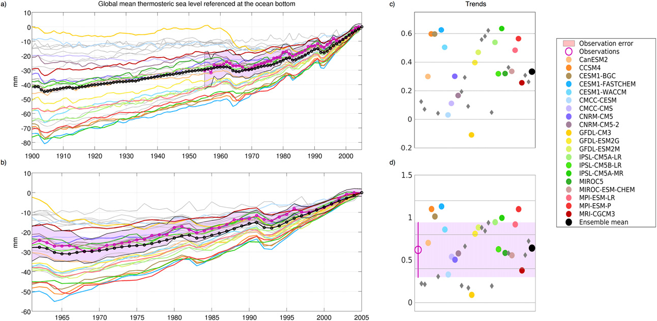 Figure 1. Thermosteric sea level (mm) and trends (mm yr-1) referenced in 2005 over (a, c) 1900–2005 and (b, d) 1961–2005.
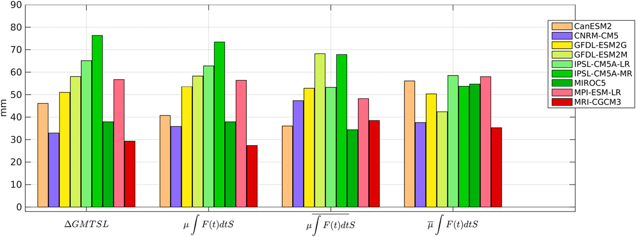
Figure 2. Thermosteric sea level rise (global mean from climate models) in 2005 relative to 1900 (mm) computed from the 3D temperature and salinity fields (first group), from the climate coefficient relationship (second group), from the climate coefficient relationship using the model ensemble mean values F (third group), and for μ (fourth group).
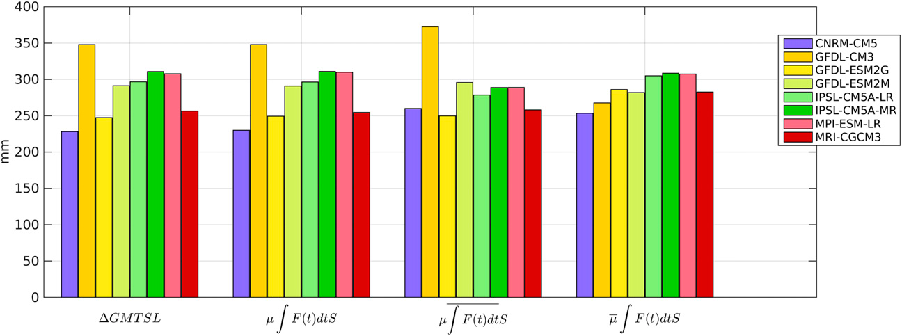
Figure 3. Thermosteric sea level rise (global mean from climate models) in 2099 relative to 2006 (mm) under the RCP8.5 IPCC scenario computed from the 3D temperature and salinity fields (first group), from the climate coefficient relationship (second group), from the climate coefficient relationship using the model ensemble mean values F (third group), and for μ (fourth group).
Links
- >>> Outreach summary in pdf
- >>> Paper in pdf – Melet A. and Meyssignac B., 2015: Explaining the Spread in Global Mean Thermosteric Sea Level Rise in CMIP5 Climate Models, J. of Climate, 28, 9918–9940