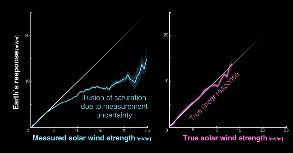









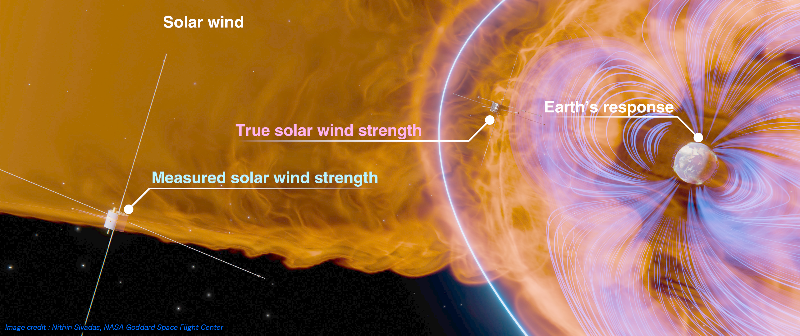
As solar wind strikes the Earth during a solar storm, electric currents are generated in the outer atmosphere. This response of the Earth to the storm, appears to level off with increasing solar wind strength measured by satellites far away from the Earth. However, Earth's response to the true solar wind that strikes the Earth, has no limit and can be greater than the apparent response. The strengths are shown in units of electric field - millivolt per meter. Image credit: Nithin Sivadas, NASA Goddard Space Flight Center
Published: 04 August 2026
New study by ISSI International Team
A Statistical Mirage in Space Weather
For more than forty years, scientists believed the Earth’s magnetic field reached a natural limit during the most powerful solar storms. This apparent “saturation” inspired ten competing physical explanations and shaped our understanding of space weather. But a new study argues that the limit never existed. Instead, it may be the product of a subtle statistical bias caused by measurement uncertainty and a phenomenon known as regression to the mean. By correcting for this bias, the researchers recover a simple linear relationship between the solar wind and the Earth’s magnetic response, overturning a long-standing assumption with implications that extend well beyond space physics.